Semantic Segmentation
Semantic segmentation is a field of computer vision, where its goal is to assign each pixel of a given image to one of the predefined class labels, e.g., road, pedestrian, vehicle, etc. By knowing the class of each pixel, one could understand the scene depicted on a given image, and the knowledge of scene understanding would help robots better navigate, without bumping into other objects, where it needs to go. This page describes an application of a fully convolutional network (FCN) for semantic segmentation.
Training a Fully Convolutional Network (FCN) for Semantic Segmentation
1. Introduction
Semantic segmentation is a computer vision task of assigning each pixel of a given image to one of the predefined class labels, e.g., road, pedestrian, vehicle, etc. If done correctly, one can delineate the contours of all the objects appearing on the input image. For object detection/recognition, instead of just putting rectangular boxes around a couple of objects, such an approach has a significant benefit over the conventional classification algorithms generating bounding boxes: An exhaustive labeling of all the pixels on a given image. This would help our robots including self-driving cars, better understand not only where they can and cannot go, but also what objects are around and make them ready about how to interact with those recognized objects.
This page will describe what the fully convolutional network is, a way of implementing it using the TensorFlow, and an application of a FCN for a pixelwise, binary classification: road or not-road -- a scale-down version of semantic segmentation.
2. Fully Convolutional Network (FCN) for Semantic Segmentation
2.1 Overview
A convolutional neural network (CNN) is typically comprised of a series of convolution layers, followed by fully connected layers and by a soft max activation function. Such architectures work really well for classification, object detection -- remember how do all these frenzies about convolutional neural network begin? Yes, at the Large Scale Visual Recognition Challenge 2012 -- ImageNet classification, the AlexNet drastically improved the classification accuracy by dropping the error rate from 26% to 15%!
 Source
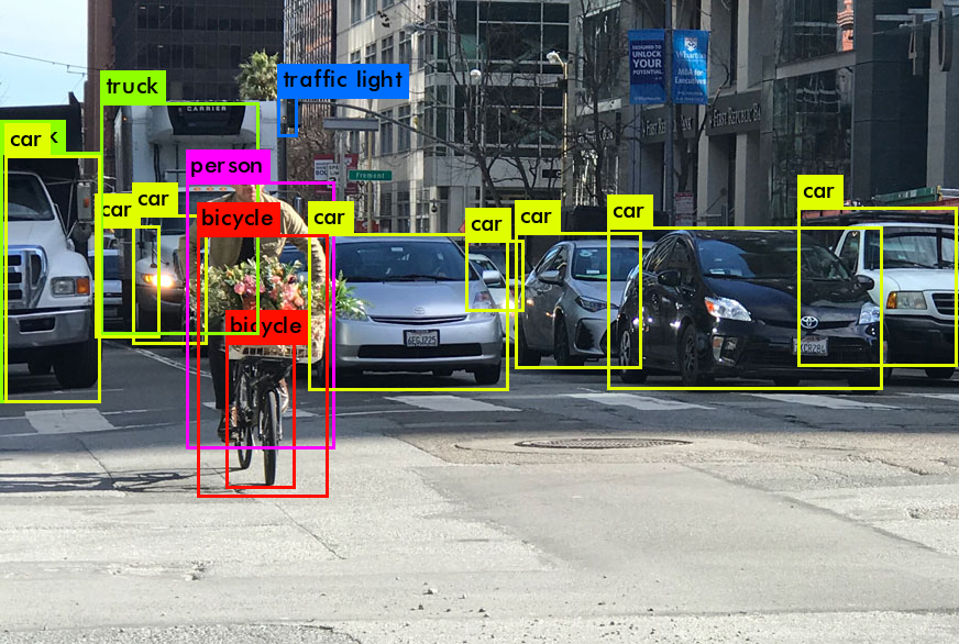
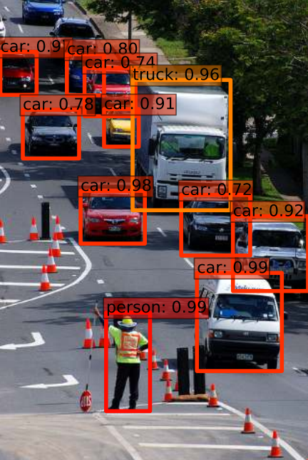
A typical output of a classification including that of the AlexNet is a bounding box around an object of interest. See examples of the bounding boxes from the above, by Yolo, and from the below, by SSD around objects like cars, bicyclist, traffic light, truck, pedestrian. These bounding boxes tells our robots what and where objects in the scene are so that they could navigate the scene without bumping into them. Of course, since a 2d image does not contain any information about distances to the detected objects, the 3d information with respect to the detected objects is assumed to be, somehow, resolved: One could use a stereo camera or fuse images with lidar points to estimate distances to the objects. There have been so many great classification and object detection algorithms developed: SVMs with HoG as a canonical example of non-DNN based, Yolo, SSD as DNN/CNN based classification/object detection algorithms, etc.
Read the following to learn more about some of the DNN-based, object detection algorithms:
 Source
But what if we want to know the positions of all the pixels delineating road's boundary, instead of the bounding boxes around image subregion about road? Does it even make sense to put a rectangle around image subregion about road? Can our awesome CNN do such a task for us? Unfortunately, no, they cannot, because the fully connected layers at the end of most of the CNNs do not preserve any spatial information. Well, then, do we have any DNN algorithm does such a task for us? Fortunately, yes, the fully convolutional network (FCN) can do it for us -- a FCN can help us assign one of the target classes to each pixel of a given image like the following:
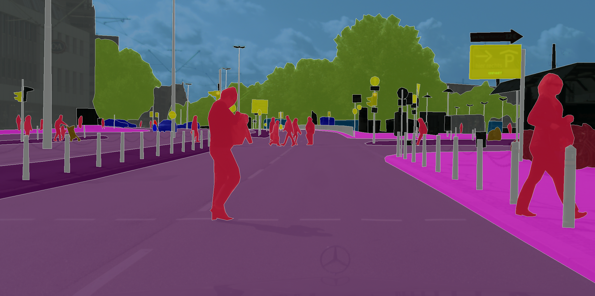
Note that the above image is not actual output of a FCN, but it's a manually labeled image used for training/testing a FCN -- it is a part of the Cityscapes dataset). We'll go into details to learn how a FCN can do such a task for us. But briefly, it can perform such a semantic segmentation because, while doing the convolution, a FCN preserve the spatial information throughout the entire network. In addition, since convolutional operations fundamentally don't care about the size of the input, a FCN will work on images in any size. In a classic convolutional network with fully connected final layers, the size of the input is constrained by the size of the fully connected layers. Passing different size images through the same sequence of convolutional layers and flattening the final output. These outputs would be of different sizes, which doesn't work very well for matrix multiplication.
Read the followings to learn more about FCN-based semantic segmentation.
- A 2017 guide to semantic segmentation with deep learning
- Fully convolution networks for 2d segmentation
- Semantic segmentation with deep learning: a guide and code
How does a FCN then accomplish such a task? It can do such a task for us primarily based on three special techniques on the top of a CNN:
- 1x1 convolutioinal layers,
- up-sampling, and
- skip connections.
A FCN is typically comprised of two parts: encoder and decoder. An encoder extracts features that will later be used by the decoder. It's common to use the encoder pre-trained on ImageNet. As examples, VGG and ResNet are popular choices. Since this is conceptually the same as a transfer learning, we can use techniques from transfer learning to accelerate the training of our FCNs. To convert a CNN into a FCN, the first thing one needs to do is to convert the fully connected layer into an 1x1 convolutional layer. And then the encoder is followed by the decoder, which uses another technique of transposed convolutional layers to upsample the image. Lastly the skip connection is added. What the skip connection does is to connect the output of one layer to a non-adjacent layer. By doing so, the skip connection allows the network to use information from multiple resolutions. While utilizing the skip connections, one'll have to be careful not to add too many skip connections. Otherwise it can lead to the explosion in the size of your model. For example, when using VGG-16 as the encoder, only the third and the fourth pooling layers are typically used for skip connections. Once we're done with incorporating all these three techniques, we can train the model end to end as we do for a CNN. Read the followings to learn more about some encoder and decoder architectures.
- SegNet: A deep convolutional encoder-decoder architecture for image segmentation
- Encoder-decoder networks for semantic segmentation
2.2 1x1 Convolution Layer
What do we mean by using 1x1 convolutional layers? It is to replace a fully connected layer of a CNN with 1x1 convolutional layers. By doing so, the output of the convolution operation is the result of sweeping the kernel over the input with the sliding window and performing element wise multiplication and summation. One way to think about this is the number of kernels is equivalent to the number of outputs in a fully connected layer. Similarly, the number of weights in each kernel is equivalent to the number of inputs in the fully connected layer. Effectively, this turns convolutions into a matrix multiplication with spatial information.
In TensorFlow, one can implement 1x1 convolutional layer by:
tf.layers.conv2d(x, num_outputs, kernel_size=1, stride=1, weights_initializer=custom_init)
where,
- num_outputs: the number of output channels or kernels
- weight initialization
- regularization
2.3 Up-Sampling
An up-sampling is done through a transposed convolution. A transposed convolution is essentially a reverse convolution where the forward and the backward passes are swapped -- this is why it is called transpose convolution. Some people call it deconvolution because it literally undoes the previous convolution. Note that the math is exactly the same because what we're doing is swapping the order of forward and backward passes.
Such transposed convolutions help in upsampling the previous layer to a higher resolution or dimension. Let's take an example: Suppose you have a 3x3 input and you wish to upsample that to the desired dimension of 6x6. The process involves multiplying each pixel of your input with a kernel or filter. If this filter was of size 5x5, the output of this operation will be a weighted kernel of size 5x5. This weighted kernel then defines your output layer. However, the upsampling part of the process is defined by the strides and the padding. In TensorFlow, using the `tf.layers.conv2d_transpose`, a `stride` of 2, and `"SAME"` padding would result in an output of dimensions 6x6. See the followings to learn more about up-sampling.
In TensorFlow,
tf.layers.conv2d_transpose(x, 3, (2, 2), (2,2))
2.4 Skip Connections
The third special technique that a FCN uses is the skip connection. One effect of convolutions or encoding in general is you narrow down the scope by looking closely at some picture and lose the bigger picture as a result. So even if we were to decode the output of the encoder back to the original image size, some information has been lost. Skip connections are a way of retaining the information easily. The way skip connection work is by connecting the output of one layer to a non-adjacent layer.
2.5 Implementation of a FCN
This section details how to implement, using TensorFlow, a fully convolutional network for a pixelwise, binary classification: road or not-road. Instead of doing a full-scale, semantic segmentation, what we do here is to implement a binary segmentation for road.
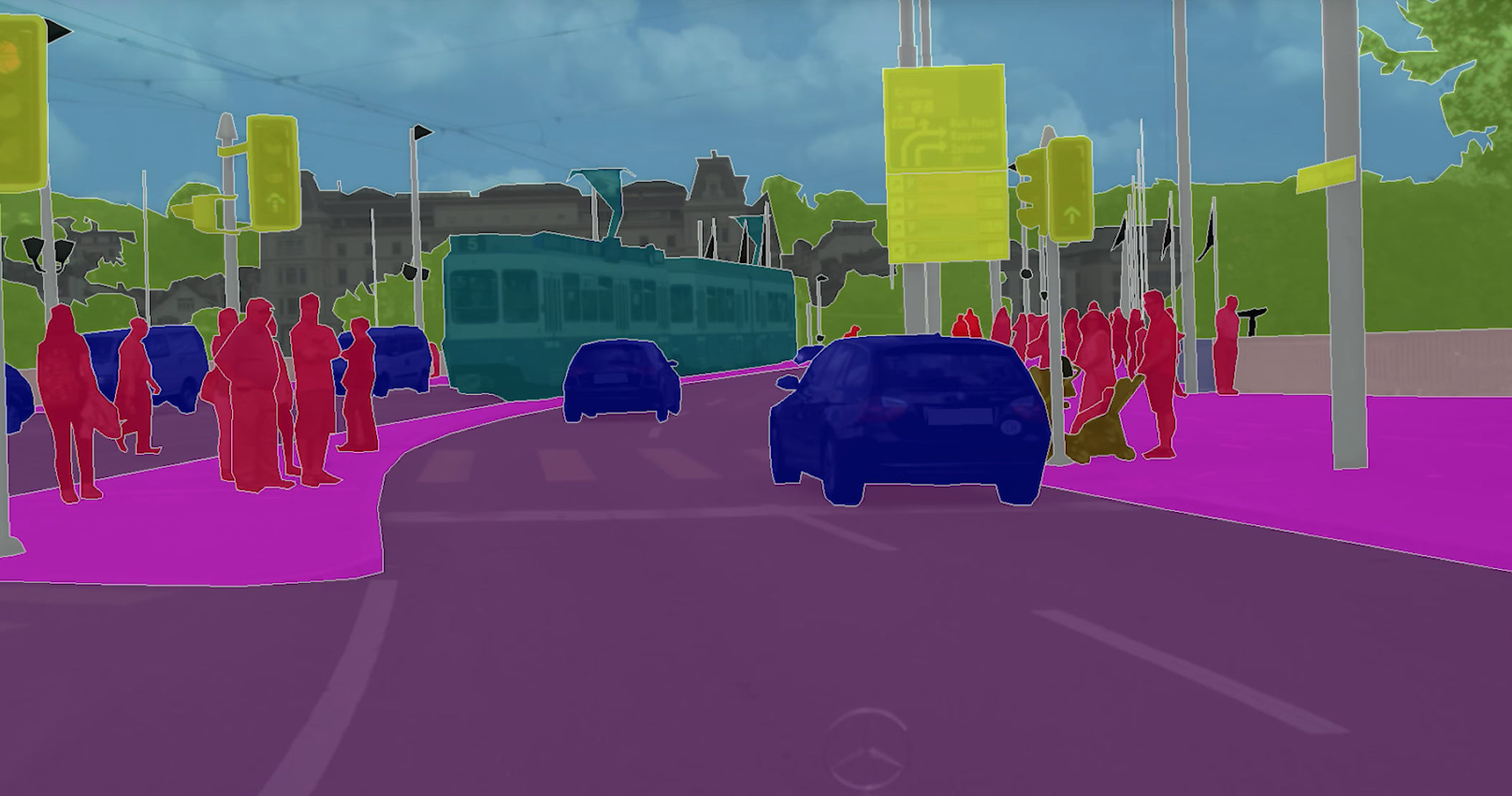
The above image is an example of the CityScapes dataset where each pixl in the image is painted with different color based on what the target class it's belonging to. The conceivable target classes include road, car, pedestrian, sign, monorail, etc. The image is generated by human annotators and used as the ground truth. Thus by doing semantic segmentation one will get valuable information about the scene appearing on the image, instead of slicing sections into bounding boxes. Semantic segmentation is also known as scene understanding, particularly for the field of autonomous driving. Read the followings to learn more about this topic.
- Fast scene understanding for autonomous driving
- ECCV-18 Workshop on Computer Vision for Road Scene Understanding and Autonomous Driving
- A survey of scene understanding by event reasoning in autonomous driving
The FCN we are primarily based on is the FCN-8. The encoder for FCN-8 is the VGG16 model pretrained on ImageNet for classification. The fully-connected layers are replaced by 1-by-1 convolutions. Here’s an example of going from a fully-connected layer to a 1x1 convolution in TensorFlow:
  num_classes = 2
  output = tf.layers.dense(input, num_classes)
To
  num_classes = 2
  output = tf.layers.conv2d(input, num_classes, 1, strides=(1,1))
To build the decoder portion of FCN-8, next we’ll have to upsample the input to the original image size. The shape of the tensor after the final convolutional transpose layer will be 4-dimensional: (batch_size, original_height, original_width, num_classes). Let’s implement those transposed convolutions we discussed earlier as follows:
output = tf.layers.conv2d_transpose(input, num_classes, 4, strides=(2,2))The transpose convolutional layers increase the height and width dimensions of the 4D input Tensor.
The final step is adding skip connections to the model. In order to do this we’ll have to combine the output of two layers. The first output is the output of the current layer. The second output is the output of a layer further back in the network, typically a pooling layer. In the following example we combine the result of the previous layer with the result of the 4th pooling layer through elementwise addition (`tf.add`).
input = tf.add(input, pool_4)We can then follow this with another transposed convolution layer.
input = tf.layers.conv2d_transpose(input, num_classes, 4, strides=(2, 2))We’ll repeat this once more with the third pooling layer output.
input = tf.add(input, pool_3)
Input = tf.layers.conv2d_transpose(input, num_classes, 16, strides=(8, 8))
Now we're done in converting a CNN, vgg16, into a FCN: converting a fully connected layer into an 1x1 convolutional layer, doing up-sampling, and skipping connections. The last step one needs to do is to define the details of training: defining the loss function. A good news is that there is nothinig special we need to do -- just training exactly same as the way we train a normal classification CNN, even with the goal of a FCN is different from that of CNN. Yes, we can still use the cross entropy loss. But one thing we have to remember the output tensor is 4D so we have to reshape it to 2D:
logits = tf.reshape(input, (-1, num_classes))where, `logits` is now a 2D tensor where each row represents a pixel and each column a class. From here we can just use standard cross entropy loss:
cross_entropy_loss = tf.reduce_mean(tf.nn.softmax_cross_entropy_with_logits(logits, labels))That's all the details we need to implement a FCN using the TensorFlow.
Now let's go into details about how the actual codes look like. Firstly we need codes that can load a pretrained vgg model.
def load_vgg(sess, vgg_path):
    """
    Load a pre-trained network, VGG for this case, into TensorFlow as an encoder.

    :param sess: TensorFlow Session
    :param vgg_path: Path to vgg folder, containing "variables/" and "saved_model.pb"

    :return: Tensors from VGG model (image_input, keep_prob, layer3_out, layer4_out, layer7_out)
    """

    vgg_tag = 'vgg16'
    vgg_input_tensor_name = 'image_input:0'
    vgg_keep_prob_tensor_name = 'keep_prob:0'
    vgg_layer3_out_tensor_name = 'layer3_out:0'
    vgg_layer4_out_tensor_name = 'layer4_out:0'
    vgg_layer7_out_tensor_name = 'layer7_out:0'

    # Use tf.saved_model.loader.load to load the model and weights
    # tf.saved_model.loader.load() returns a protobuf
    tf.saved_model.loader.load(sess, [vgg_tag], vgg_path)

    # Get tensors to return
    image_input = sess.graph.get_tensor_by_name(vgg_input_tensor_name)
    keep_prob = sess.graph.get_tensor_by_name(vgg_keep_prob_tensor_name)
    layer3_out = sess.graph.get_tensor_by_name(vgg_layer3_out_tensor_name)
    layer4_out = sess.graph.get_tensor_by_name(vgg_layer4_out_tensor_name)
    layer7_out = sess.graph.get_tensor_by_name(vgg_layer7_out_tensor_name)

    return image_input, keep_prob, layer3_out, layer4_out, layer7_out's
After we load a pre-trained vgg, what we do next is, in order to create a FCN, to 1) convert a fully connected layer into 1x1 convolutional layer, 2) do up-sampling and 3) skip connections.
def layers(vgg_layer3_out, vgg_layer4_out, vgg_layer7_out, num_classes):
    """
    Create a fully convolutional network, using the vgg layers, with 1x1
    convolution, skip-connection, transpose for upsampling

    :param vgg_layer3_out: TF Tensor for VGG Layer 3 output
    :param vgg_layer4_out: TF Tensor for VGG Layer 4 output
    :param vgg_layer7_out: TF Tensor for VGG Layer 7 output
    :param num_classes: Number of the target classes

    :return: The Tensor for the last layer of output

    """

    # Given a pre-trained network (VGG) as encoder

    # A function, from the class, for creating 1x1 convolution layer
    def conv_1x1(x, num_outputs):
        kernel_size = 1
        stride = 1
        # regularization makes output much appealing!
        return tf.layers.conv2d(x, num_outputs, kernel_size, stride,
                                kernel_initializer=tf.truncated_normal_initializer(stddev=0.01),
                                kernel_regularizer = tf.contrib.layers.l2_regularizer(1e-3))

    # num_outputs/kernels should be the same as
    # num_classes. num_classes should be 2 for this project -- a
    # binary classification: road or non-road?
    conv_out = conv_1x1(vgg_layer7_out, num_classes)

    # Transposed/backward convolutions for creating a decoder
    deconv_1 = tf.layers.conv2d_transpose(conv_out, num_classes, 4, 2, 'SAME',
                                          kernel_initializer=tf.truncated_normal_initializer(stddev=0.01),
                                          kernel_regularizer = tf.contrib.layers.l2_regularizer(1e-3))

    # Add a skip connection to previous VGG layer
    skip_layer_1 = conv_1x1(vgg_layer4_out, num_classes)
    skip_conn_1 = tf.add(deconv_1, skip_layer_1)

    # Up-sampling
    deconv_2 = tf.layers.conv2d_transpose(skip_conn_1, num_classes, 4, 2, 'SAME',
                                          kernel_initializer=tf.truncated_normal_initializer(stddev=0.01),
                                          kernel_regularizer = tf.contrib.layers.l2_regularizer(1e-3))

    # Add another skip connection to previous VGG layer
    skip_layer_2 = conv_1x1(vgg_layer3_out, num_classes)
    skip_conn_2 = tf.add(deconv_2, skip_layer_2)

    # Up-sampling again
    deconv_3 = tf.layers.conv2d_transpose(skip_conn_2, num_classes, 16, 8, 'SAME',
                                          kernel_initializer=tf.truncated_normal_initializer(stddev=0.01),
                                          kernel_regularizer = tf.contrib.layers.l2_regularizer(1e-3))

    return deconv_3
Once we complete to define the structure of the FCN, we need to define a setup for training a neural network.
def optimize(nn_last_layer, correct_label, learning_rate, num_classes):
    """
    Optimize the fcn by defining the loss function and the optimization method.

    :param nn_last_layer: TF Tensor of the last layer in the neural network
    :param correct_label: TF Placeholder for the correct label image
    :param learning_rate: TF Placeholder for the learning rate
    :param num_classes: Number of classes to classify

    :return: Tuple of (logits, train_op, cross_entropy_loss)
    """

    # Reshape predictions and labels through flattening
    logits = tf.reshape(nn_last_layer, (-1, num_classes))
    labels = tf.reshape(correct_label, (-1, num_classes))

    # Define the loss function
    cross_entropy_loss = tf.reduce_mean(tf.nn.softmax_cross_entropy_with_logits(labels=labels, logits=logits))

    # Define optimizer, ADAM
    optimizer = tf.train.AdamOptimizer(learning_rate=learning_rate)

    # Define train_op to minimise loss
    train_op = optimizer.minimize(cross_entropy_loss)

    return logits, train_op, cross_entropy_loss
Now we need to define the procedure of training a neural network.
def train_nn(sess, epochs, batch_size, get_batches_fn, train_op, cross_entropy_loss, input_image,
             correct_label, keep_prob, learning_rate):
    """
    Train the fcn.

    :param sess: TF Session
    :param epochs: Number of epochs
    :param batch_size: Batch size
    :param get_batches_fn: Function to get batches of training data.  Call using get_batches_fn(batch_size)
    :param train_op: TF Operation to train the neural network
    :param cross_entropy_loss: TF Tensor for the amount of loss
    :param input_image: TF Placeholder for input images
    :param correct_label: TF Placeholder for label images
    :param keep_prob: TF Placeholder for dropout keep probability
    :param learning_rate: TF Placeholder for learning rate
    """

    # define hyper-parameters
    keep_prob_stat = 0.8
    learning_rate_stat = 1e-4

    for epoch in range(epochs):
        for image, label in get_batches_fn(batch_size):
            _, loss = sess.run([train_op, cross_entropy_loss],
                               feed_dict={input_image: image,
                                          correct_label: label,
                                          keep_prob: keep_prob_stat,
                                          learning_rate:learning_rate_stat})

        print("Epoch %d of %d: Training loss: %.4f" %(epoch+1, epochs, loss))
Now we have everything: architecture, how to train and a training procedure. Let's put everything together.
#!/usr/bin/env python3
import tensorflow as tf

def run():
    num_classes = 2
    image_shape = (160, 576)
    data_dir = './data'
    runs_dir = './runs'

    tests.test_for_kitti_dataset(data_dir)

    # Set hyper-parameters
    epochs = 20
    batch_size = 1

    # Download the pretrained vgg model
    helper.maybe_download_pretrained_vgg(data_dir)

    with tf.Session() as sess:
        # Path to vgg model
        vgg_path = os.path.join(data_dir, 'vgg')

        # Create function to get batches
        get_batches_fn = helper.gen_batch_function(os.path.join(data_dir, 'data_road/training'), image_shape)

        # Build NN using load_vgg, layers, and optimize function
        image_input, keep_prob, vgg_layer3_out, vgg_layer4_out, vgg_layer7_out = load_vgg(sess, vgg_path)

        # Build a FCN
        last_layer = layers(vgg_layer3_out, vgg_layer4_out, vgg_layer7_out, num_classes)

        correct_label = tf.placeholder(dtype=tf.float32, shape=(None, None, None, num_classes))
        learning_rate = tf.placeholder(dtype=tf.float32)

        # Make optimization ready
        logits, train_op, cross_entropy_loss = optimize(last_layer, correct_label, learning_rate, num_classes)

        # Train the fcn using the train_nn function
        sess.run(tf.global_variables_initializer())
        train_nn(sess, epochs, batch_size, get_batches_fn, train_op, cross_entropy_loss, image_input,
                 correct_label, keep_prob, learning_rate)

if __name__ == '__main__':
    run()
3. Results
This section explains how to run the above explained code and reviews some results. The first order business is to make your machine ready for the task by installing all the necessary packages.
3.1 Setup
In order to make the above described code run, you'll need a GPU or some of them. If your machine doesn't have any fancy Nvidia's GPU boards, you might want to consider to use GPU-enabled cloud service like AWS or other equivalents. See the following to learn how to set up AWS EC (Elastic Compute).
- Setting up with Amazon EC2
- Getting started with Amazon EC2 linux instances
- AWS EC2 tutorial for beginners
- Deep Learning AMI
For either your local machine or the host machine on a cloud service, the list of the packages you'll need to install:
3.2 Dataset
There is a couple of semantic segmendataion datasets available, particularly, for autonomous driving.
For this experiment, we used the KITTI road dataset.3.3 Training
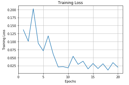
For the training, I used an AMI, a gpu instance of g2.8xlarge (vCPUs: 32, Memory: 60GiB, $0.8424) from AWS about one and half hour to run the above-described FCN. Some of the hyperparameters include
- epochs: 20,
- learning rate: 1e-4,
- keeping probability: 0.8,
- batch size: 1 (for the AMI I used, the code didn't run unless the batch size is 1. Otherwise it stopped by spitting "Resource Exhausted" error's),
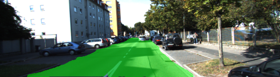
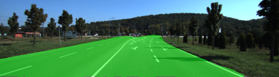
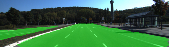
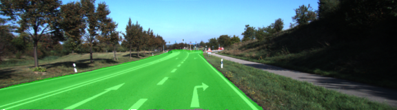
3.4 Results of Road-Region Classification
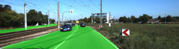
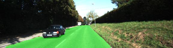
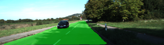
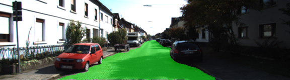
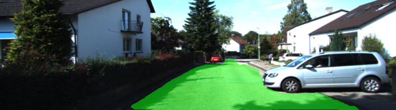
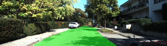
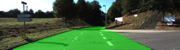
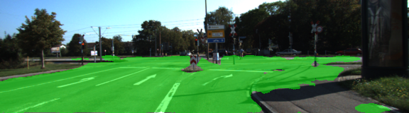
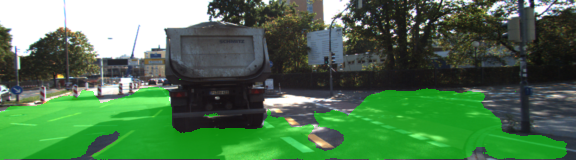
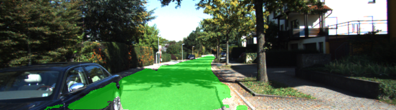
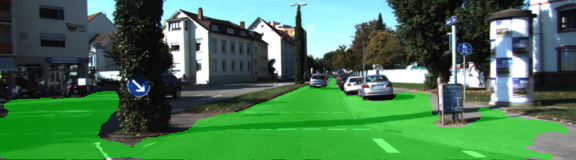
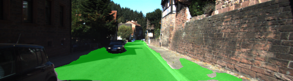
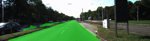
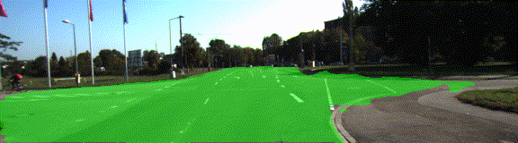
Let's take a look at some results where the segmentation worked reasonably well. Note that at the moment I wasn't able to compute any quantitative analysis (like IoU) on the results due to unavailability of the ground-truth or my laziness. So, we're qualitatively evaluating the performance. Take a close look at those testing images where parts of road, image subregions are covered by shade.
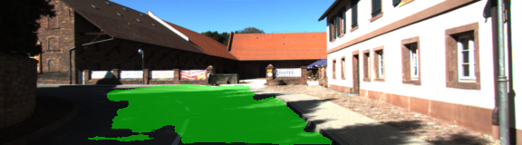
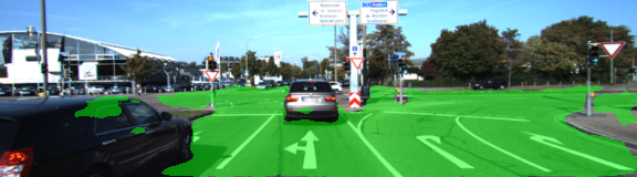
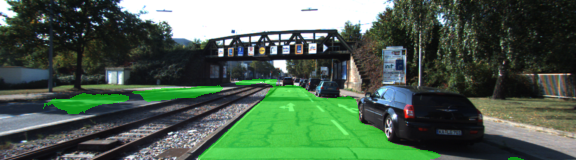
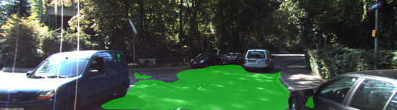
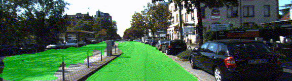
Now let's look at some examples that the segmentation didn't work very well. Anyone can easily spot missegmented regions: shade, pedestrian road, part of cars, etc.
The following animated images at the below show all of the segmentation results altogether -- results of a pixel-wise, binary classification.
4. Summary
This page describes what semantic segmentation is, what a fully convolutional network (FCN) is and how it is used for semantic segmentation -- a binary classification of roads. In particular, I describe
- What is semantic segmentation,
- How a FCN is built from a CNN by utilizing 1x1 convolutional layer, transposed convolution for up-sampling, skip connections,
- How one can implement a FCN using TensorFlow, and
- Application of FCN to semantic segmentation.